
Consensus Based Optimization
\[\newcommand{\N}{\mathbb{N}} \newcommand{\R}{\mathbb{R}} \newcommand{\Rd}{\mathbb{R}^d} \newcommand{\d}{d} \newcommand{\kernel}{\mathsf{k}} \newcommand{\mean}{\mathsf{m}} \newcommand{\kmean}{\mean_{\kernel}} \newcommand{\wkmean}{\mean_{\kernel}} \newcommand{\abs}[1]{\left|#1\right|}\]Setting
We consider a function $V:\R^d\to\R^+_0$ for which we want to solve the global optimization problem
\[\min_{x\in\R^d} V(x).\]-
The function $V$ may be non-convex.
-
We do not want to employ gradient-based methods.
-
Instead: agent based/particle methods.
Particle Swarm Optimization
We first consider Particle Swarm Optimization (PSO) proposed by Kennedy and Eberhart (1995) which was motivated by bird-flocking simulations of Reynolds (1987).
For particles $x_1,\ldots, x_N\in\R^d$ with velocities $v_i\in\R^d$ one considers the scheme
\[\begin{align*} x_i &\gets x_i + v_i,\\ v_i &\gets v_i + \xi_1\circ (p_i - x_i) + \xi_2 \circ (p_\text{g} - x_i). \end{align*}\]Here,
- $\xi_1, \xi_2\in\R^d$ are chosen randomly,
- $p_i\in\R^d$ denotes the best position particle $i$ has seen,
- $p_\text{g}$ denotes the best the swarm has seen.
Consensus
The first step to derive standard CBO proposed by Pinnau (2017) is to only consider a common point $\mean\in\Rd$. Secondly, this point is chosen as the weighted average
\[\mean[\rho^N] = \frac{\int y\ \exp(-\beta\ V(y)) d\rho^N(y)}{\int \exp(-\beta\ V(y)) d\rho^N(y)}\]where $\rho^N = \sum_{i=1}^N \delta_{x_i}$.
For $i=1,\ldots,N$ the dynamics then read
\[\begin{align*} \boxed{ \dot{x}_i = -(x_i - \mean[\rho^N]) + \sigma \abs{x_i - \mean[\rho^N]}\dot{W_i}, } \end{align*}\]where the parameter $\sigma \geq 0$ determines the influence of the noise term. Considering the mean-field equation (formally) one obtains the dynamic
\[\dot{x} = -(x - \mean[\rho]) + \sigma \abs{x - \mean[\rho]}\dot{W_i},\qquad \rho = \text{law}(x)\]Modifications and Details
-
The parameter $\beta$ is typically updated during the iteration.
-
Especially for higher-dimensional problems Carillo et al. (2018) proposed a noise term that is scaled component-wise.
-
Carillo et al. (2018) also proposed a batching strategy over the particles.
-
In some formulations the term $(x_i - \mean)$ is multiplied by a term that enforces an improvement in every step.
Kernelized CBO
The standard CBO scheme does not incorporate a “personal best” like PSO schemes.
-
CBO does does not allow to find multiple global minima,
-
it has been empirically observed \cite{totzeck_20} that CBO performs worse for certain initializations.
How can we modify the scheme to incorporate a “personal best” like in the PSO case?
A possible method was proposed by Totzeck et al (2020) who introduced a weighted average over time
\[\begin{align*} p_i(t) := \frac{\int_0^t x_i(s)\ \exp(-\beta\ V(x_i(s))) ds}{\int_0^t \exp(-\beta\ V(x_i(s))) ds}. \end{align*}\]Our approach employs a spatial localization in the state space.
Modification of CBO: Introducing a Kernel
The weighted mean $\mean$ for CBO
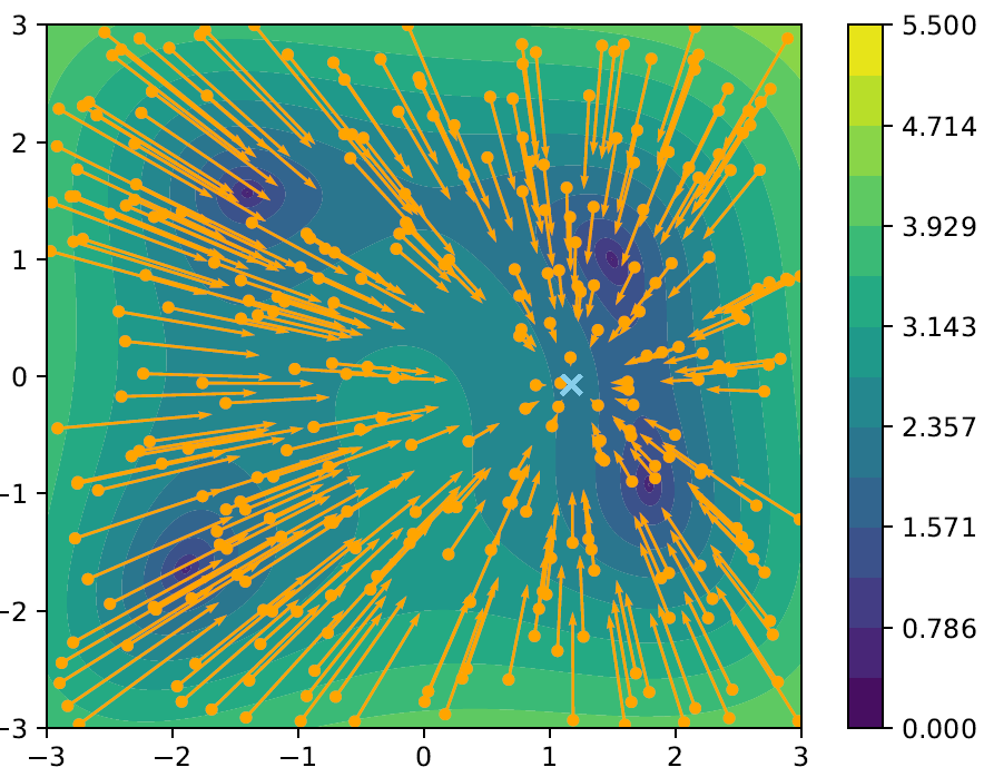
\[\begin{align*} \mean[\rho] := \frac{\int y \exp(-\beta V(y))\d\rho(y)}{\int \exp(-\beta V(y))\d\rho(y)}. \end{align*}\]induces a vector field $x\mapsto \mean[\rho] - x$ that points towards $\mean[\rho]$ globally.
Introducing a kernel $\kernel:\R^d\times\R^d\to\R$
\[\begin{align*} \kmean[\rho](x) := \frac{\int\kernel(x,y)\ y \exp(-\beta V(y))\d\rho(y)}{\int \kernel(x,y)\exp(-\beta V(y))\d\rho(y)} \end{align*}\]allows for $x\mapsto x-\kmean[\rho] (x)$ to be non-affine.
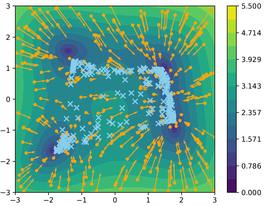
The modified update scheme then has the form
\[\begin{align*} \dot x_i = -(x_i - \wkmean[\rho](x_i)) + \sigma\abs{x_i - \wkmean[\rho](x_i)}\dot W_i, \qquad \rho := \sum_{i=1}^N\delta_{x_i}. \end{align*}\]Note: Every particle $x_i$ now (possibly) has a personal average.
CBO via Expectation maximization
A possible choice to evaluate the kernel $\kernel$ is to perform clustering on the particles in every update step.
To do so we assume a Gaussian mixture model with $M$ components
\[\begin{align*} (\mu^1, \ldots, \mu^M)\\ (\Sigma^1, \ldots, \Sigma^M) \end{align*}\]and define
\[\begin{align*} q_{i,k} := \frac{\exp(\varphi(x_i; \mu^k, \Sigma^k))}{\sum_{j=1}^M \exp(\varphi(x_i; \mu^k, \Sigma^k))} \end{align*}\]where $x\mapsto \varphi(x; \mu, \Sigma)$ denotes the PDF with mean $\mu$ and covariance matrix $\Sigma$. With this we can set
\[\begin{align*} m^k = \frac{\sum_{i=1}^N x_i\ q_{i,k}\ \exp(-\beta\ V(x_i))}{\sum_{i=1}^N q_{i,k}\ \exp(-\beta\ V(x_i))} \end{align*}\]and therefore
\[\begin{align*} \boxed{ \kmean[\rho^N](x_i) = \sum_{k=1}^M q_{i,k} m^k.} \end{align*}\]

CBO via Clustering
A related approach is to determine the kernel via Clustering. For given particles $x_1,\ldots, x_N$ we determine $M\in\N$ clusters $C_1,\ldots,C_M$ and set
\[\begin{align*} m_k := \frac{\sum_{j\in C_k} x_j \exp(-\beta\ V(x_j))}{\sum_{j\in C_k} \exp(-\beta\ V(x_j))} \end{align*}\]as the weighted average of each cluster. We then set
\[\begin{align*} \boxed{ \kmean[\rho^N](x_i) := m_{k(i)}} \end{align*}\]where $k(i)\in{1,\ldots,M}$ denotes the index such that $x_i\in C_{k(i)}$, which is equivalent to choosing the kernel
\[\begin{align*} \kernel(x,y) = \begin{cases} 1 &\text{ if } x,y\in C_k \text{ for one } k\in\{1,\ldots, M\},\\ 0 &\text{ else}. \end{cases} \end{align*}\]
Distance Based CBO
Alternatively one can replace the clustering approach, by simply considering the Euclidean distance of the particles, e.g., choosing
\[\begin{align*} \kernel(x,y) = \exp\left(-\frac{\abs{x- y}^2}{2\kappa^2}\right). \end{align*}\]Here, $\kappa\geq 0$ controls the length scale of the particle communication,
- for $\kappa=0$ every particle only communicates with itself,
- for $\kappa=\infty$ we recover standard CBO.
The weighted mean, then has the form
\[\begin{align*} \kmean[\rho](x) := \frac{\int y \exp\left(- \frac{\abs{x-y}^2}{2\kappa^2} -\beta V(y) \right)\d\rho(y)}{\int \exp\left(- \frac{\abs{x-y}^2}{2\kappa^2}-\beta V(y) \right)\d\rho(y)}. \end{align*}\]

Modifications
Especially in a higher-dimensional it can be better to again consider the mean focused approach. I.e., we have $M\in\N$ different points $m^1,\ldots, m^M\in\Rd$ and update them via
\[\begin{align*} q_{i,k} := \frac{\exp\left(- \frac{\abs{m^k-x_i}^2}{2\kappa^2} \right)}{\sum_{j=1}^M \exp\left(- \frac{\abs{m^k-x_i}^2}{2\kappa^2} \right)} \\ m^k \gets \frac{\sum_{i=1}^N x_i\ q_{i,k}\ \exp(-\beta\ V(x_i))}{\sum_{i=1}^N q_{i,k}\ \exp(-\beta\ V(x_i))}. \end{align*}\]With these points we can again choose
\[\begin{align*} \kmean[\rho](x_i) := \sum_{k=1}^M q_{i,k} {m^k} \end{align*}\]Higher-Dimensional Example
Let $U:\R^d\to\R^+_0$ denote the Ackley function
\[\begin{align*} U(x) := -20 \exp\left(-\frac{0.2}{\sqrt{d}} \abs{x}\right) - \exp\left(\frac{1}{d}\sum_{i=1}^d\cos(2\pi x_i)\right) + 20 + e, \end{align*}\]and for $\alpha_1,\ldots,\alpha_s \in\R, z_1,\ldots, z_s\in\Rd$ we consider
\[\begin{align*} V(x) = \prod_{i=0}^s U(\alpha_i x + z_i) \end{align*}\]which yields a toy problem in higher dimensions.
References
[1] Kennedy, J. and Eberhart, R. (1995). Particle swarm optimization Proceedings of ICNN’95 - International Conference on Neural Networks